Nonlinear Functions

In Gurobi, you can express various types of nonlinear relations (integrality, quadratic, …). By abuse of terminology, we refer to nonlinear functions as those relations that involve continuous nonlinear functions such as logarithm, exponential, sine, cosine, etc. These functions are used to build nonlinear expressions, from which nonlinear constraints and nonlinear objectives can be built. This section describes how nonlinear expressions are represented in Gurobi.

The optimizer offers two approaches to solving models with nonlinear objectives or constraints, selected via the OptimalityTarget parameter:

• Global optimality: a spatial branch-and-bound framework searches the feasible space and provides a globally valid objective bound. A solution is proven globally optimal (subject to tolerances) when the optimality gap is closed.

• Local optimality: the nonlinear barrier solver finds a locally optimal solution satisfying first-order optimality conditions. This option is only available for continuous models (no discrete variables or SOS constraints) and requires differentiable functions; refer to OptimalityTarget for details.

Expression Trees

Gurobi supports nonlinear expressions of the form \(f(x)\) where \(f: \mathbf{R}^n \rightarrow \mathbf{R}\) is given by an expression tree. Such trees are used to represent nonlinear objectives and constraints. The tree encodes how the function \(f\) is composed of various elementary operations, like arithmetic operations and univariate functions. We’ll discuss both concepts next.

Note

If you use Python, we recommend using arithmetic operators and our nonlinear function helpers to build nonlinear expressions (see NLExpr for details). Constructing these expressions as described here is considered advanced usage.

Let’s start with a simple example to illustrate the concept. Consider the multivariate expression \(\sin(2.5 x_1) + x_2\). The elementary operations in this expressions are multiplication, addition and the sine function. The dependencies and order of operations are as follows: On the top level there is an addition of the terms \(\sin(2.5 x_1)\) and \(x_2\). The first part decomposes into a sine function which depends on the product of the constant \(2.5\) and the variable \(x_1\). Orienting edges along the flow of data we arrive at the following representation:

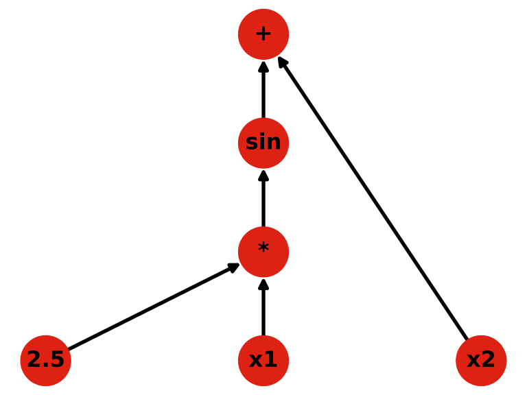
In order to pass such a directed tree to any of Gurobi’s APIs except for Python, we need to encode it with native data types. Speaking abstractly, our format uses three arrays to represent such an expression tree, where the three i-th entries together define the i-th node in the tree. The three arrays contain the following information:

• The opcode (“operation code”) array. It contains the information which elementary operation this node represents. A list of possible opcode values is given further below.

• The data array. It contains auxiliary information for this node, like the value of a constant, or the index of a variable in the optimization model. Fill a value of -1 if the corresponding opcode does not assume additional data.

• The parent array. It defines the tree topology by providing the index of this node’s parent in the array representation. The (unique) root node of the tree must have the value -1 as its parent.

The nodes of the tree must be presented in these arrays in pre-order, that is, each node of the tree must be followed by all its descendants in a consecutive manner.

Continuing our \(\sin(2.5 x_1) + x_2\) example from above, the three arrays would contain the following data:

array index	opcode	data	parent
0	plus	-1	-1
1	sin	-1	0
2	multiply	-1	1
3	constant	2.5	2
4	variable	1	2
5	variable	2	0

Let’s discuss the table line-by-line.

• Index 0: This is the root node of the tree (its parent value is -1), and it represents a “plus” operation. It doesn’t need additional data, hence its data value is set to -1.

• Index 1: This is the first child of its parent at index 0, and it represents an application of the sine function. It doesn’t need additional data, hence its data value is set to -1.

• Index 2: This is the child of its parent sine node (parent value is 1), and represents a “multiply” elementary operation. It doesn’t need additional data, hence its data value is set to -1.

• Index 3: This is the first child of its parent multiply node (parent value is 2) and represents the constant value 2.5, which is stored as the data value.

• Index 4: This is the second child of its parent multiply node (parent value is 2), and represents the variable \(x_1\) which has the index 1 in the model, as designated by the corresponding value in the data array.

• Index 5: This is the second child of its parent plus node (parent value is 0), and represents the variable \(x_2\) which has the index 2 in the model, as designated by the corresponding value in the data array.

Operation Codes

An operation code (“opcode”) describes an elementary operation that maps input values to an output value. As seen in Expression Trees, each node in an expression tree carries exactly one opcode, and we will discuss all available opcodes now.

OPCODE_CONSTANT

This opcode will “load” a constant value as an argument for its parent node. The value is specified by the corresponding entry in the data array. It cannot be a parent of a node in an expression tree.

OPCODE_VARIABLE

This opcode will “load” a variable as an argument for its parent node. The variable index is specified by the corresponding entry in the data array. Note that in some languages you may need to cast the variable index, which is an integer type, to a floating point value. It cannot be a parent of a node in an expression tree.

OPCODE_PLUS

This n-ary opcode will evaluate to the sum of all its arguments. It can have an arbitrary number of arguments, where a single argument operation amounts to a unary plus (a no-op), and an evaluation with zero arguments results in the value 0.0.

OPCODE_MINUS

This opcode is a binary operation and will evaluate to the difference of its first and second argument.

OPCODE_MULTIPLY

This n-ary opcode will evaluate to the product of all its arguments. It can have an arbitrary number of arguments, where a single argument operation amounts to a unary multiplication (a no-op), and an evaluation with zero arguments results in the value 1.0.

OPCODE_DIVIDE

This opcode is a binary operation and will evaluate to the quotient of its first argument (dividend) and second argument (divisor), viz. \(\frac{x}{y}\). Gurobi will implicitly prevent the divisor \(y\) to take values in the interval \([-10^{-10}, 10^{-10}]\).

OPCODE_UMINUS

This unary opcode evaluates to the negative of its sole argument.

OPCODE_SQUARE

This unary opcode evaluates to the square of its sole argument.

OPCODE_SQRT

This unary opcode evaluates to the square root of its sole argument. Gurobi will implicitly enforce a lower bound of zero on the argument.

OPCODE_SIN, OPCODE_COS, OPCODE_TAN

Unary opcodes for the trigonometric functions sine, cosine and tangent.

OPCODE_POW

This binary opcode evaluates to \(x^y\), where the base \(x\) is the first argument, and the exponent \(y\) is its second argument. A number of restrictions apply to this opcode:

• One of \(x\) and \(y\) must evaluate to a constant. More precisely, if Gurobi’s presolve algorithm cannot determine that either the base or the exponent evaluates to a constant, the optimization will stop with an error.

• If the base evaluates to a constant, that constant must be strictly greater than zero. Otherwise the optimization will stop with an error.

• If the exponent evaluates to a constant negative integer value, then Gurobi will implicitly prevent the base \(x\) to take values in the interval \([-10^{-10}, 10^{-10}]\).

• If the exponent evaluates to a constant nonnegative fractional value, then Gurobi will implicitly enforce a lower bound of \(0\) on the base.

• If the exponent evaluates to a constant negative fractional value, then Gurobi will implicitly enforce a lower bound of \(10^{-10}\) on the base.

OPCODE_EXP

This unary opcode evaluates to the exponential \(y\) of its sole argument \(x\), viz. \(y = \exp(x) = e^x.\)

OPCODE_LOG, OPCODE_LOG2, OPCODE_LOG10

These unary opcodes will evaluate to the logarithm (with bases \(e\), 2, and 10) of its argument. Gurobi will enforce a lower bound of \(10^{-10}\) on the argument.

OPCODE_LOGISTIC

This unary function will evaluate its argument \(x\) to the value \(y\) of the standard logistic function, viz. \(y = \frac{1}{1 + \exp(-x)}\).

OPCODE_TANH

This unary function will evaluate its argument \(x\) to the value \(y\) of the standard hyperbolic tangent function, viz. \(y = \tanh(x)\).

OPCODE_SIGNPOW

This binary opcode evaluates to \(\text{sign}(x)|x|^a\), where the base \(x\) is its first argument, and the exponent \(a \in \mathbb{R}_{\geq 1}\) is its second argument. \(\text{sign}(x)\) denotes the sign of \(x\). For example, \(\text{signpow}(x, 2) = x |x|\).

A compact reference overview of all opcodes is given in Nonlinear Operation Codes.